Closet Indexing Analysis: Python Snippets for Assessing Active Managers

Actively managed funds typically charge higher fees than index funds based on the premise that the managers’—and their investment teams’—efforts generate excess returns or alpha. 

How well do active managers deliver on that premise?  

Investment style analysis can assess the impact of manager decisions. Copy and paste for a deep dive into closet indexing and market timing ability. 

For more real-life case studies and examples, download the style analysis guide.

Closet indexing, or mimicking an index under the guise of active management, is a misleading practice that can cost investors in the long run.  

Sometimes, active funds may successfully generate alpha relative to the broad market or even the Fama-French 3 Factor model. However, it’s possible that the “alpha” might be exposure to one of these priced factors. Investors could achieve the same results with a low-cost, tax-friendly ETF without the added expenses of active management. 

Style analysis can help uncover potential closet indexing. Implement the statistical tests below. We’ll use the Morningstar Python package as our data source. 

The Morningstar data Python package gives data scientists, quants, and engineers convenient access to Morningstar data and the flexibility to use it in their preferred coding environments. To use the Python package, start by logging into Analytics Lab to retrieve your authentication token. Access full instructions on the developer site.

INPUT 

import morningstar_data as md 

import matplotlib.pyplot as plt 

import numpy as np 

import pandas as pd 

import statsmodels.formula.api as smf 

Let’s focus on actively managed mutual funds. To make the analysis manageable, limit the dataset to equity funds that:  

• Have at least USD 1 billion in total assets. 

• Have more than 5 years of live track record. 

• Charge fees higher than their Morningstar Category average. 

• Are both domiciled and invest in the United States, exclusively. 

Finally, limit the search to only one share class per fund. With this set of conditions, or filters, you can formulate the universe as a Search Criterion. For easier analysis, you could also use Morningstar Direct’s visual interface to search for relevant funds. 

INPUT 

criteria = { 

    "universeId": "FO",              # Universe is limited to Open-end funds 

    "subUniverseId": "", 

    "subUniverseName": "", 

    "securityStatus": "activeonly",  # Surviving funds only 

    "useDefinedPrimary": True,       # Only one share class per fund 

    "criteria": [ 

        {"relation": "", "field": "OF00C", "operator": "=", "value": "0"},             # Index Fund = False 

        {"relation": "AND", "field": "OF009", "operator": ">", "value": "1000000000"}, # Fund Size USD >= $1 billion 

        {"relation": "AND", "field": "LS017", "operator": "=", "value": "USA"},        # Domicile is USA 

        {"relation": "AND", "field": "OS05P", "operator": ">", "value": "CAT AVG"},    # Prospectus Net Expense Ratio higher than category average 

        {"relation": "AND", "field": "OF035", "operator": "=", "value": "$BCG$EQUTY"}, # Broad asset class is equity 

        {"relation": "AND", "field": "OS00F", "operator": "<=", "value": "04/30/2019"},# Inception on or before Apr 30, 2019 

        {"relation": "AND", "field": "OS63Z", "operator": "=", "value": "AREA$$$NAU"}, # Area of investment is USA i.e., non-international funds 

    ] 

} 

INPUT 

fund_list = md.direct.get_investment_data(investments=criteria, data_points=[{"datapointId": "OS01W"}, {"datapointId": "OS00I"}, {"datapointId": "OS385"}]) 

fund_list.head(3) 

OUTPUT

INPUT 

len(fund_list) 

OUTPUT

394 

Now that you’ve identified nearly 400 candidate funds, obtain five years of monthly returns for these funds to use in the regression models. This snippet uses the Python package.

INPUT 

%time 

fund_returns_raw = md.direct.get_returns( 

    investments=fund_list['SecId'].tolist(), 

    start_date='2019-06-30', 

    end_date='2024-05-31' 

) 

fund_returns_raw.head(3) 

OUTPUT 

Pivot the returns into a wide format. 

INPUT 

fund_returns_wide = ( 

    fund_returns_raw 

    .pivot( 

        index='Date',  

        columns='Id',  

        values='Monthly Return' 

    ) 

    .div(100) 

) 

fund_returns_wide.head(3) 

OUTPUT

3 rows x 394 columns

Now load the factor premia. This snippet uses premia from the Morningstar North America Standard Risk Model. The model goes beyond the Fama-French alternative to consider additional factors like: 

• Liquidity, or how well a fund can meet cash flow demands. 

• Volatility, or variations in returns. 

• Yield, or the income generated by an investment. 

• Quality. High-quality firms have high profitability and low financial leverage. 

INPUT 

mstar_premia_raw = pd.read_csv('mstar-NA-premia.csv') 

mstar_premia_raw.head(3) 

OUTPUT 

Format to set the date as an index and decimalize by dividing by 100. 

INPUT 

mstar_premia = ( 

    mstar_premia_raw 

    .assign(Date=lambda x: pd.to_datetime(x.Date)) 

    .set_index('Date') 

    .div(100) 

OUTPUT 

With all the information loaded, focus on experimentation. Let’s perform a simple test. 

1. Train a multivariate linear regression model with the fund returns on the LHS and the factor model on the RHS. 

2. Observe the goodness of fit of the model via its F-statistic. 

3. Note the R-squared of all well-fit models. 

Funds with very high R-squared values are those where the entire variation in returns can be explained by systematic risk factors. Since such exposure should be cheap, investors shouldn’t have to pay high fees for these funds. 

First, create three empty lists to store funds. 

INPUT

rsq_95 = [] 

rsq_98 = [] 

rsq_99 = [] 

Fetch the available fund return dates, available premia dates, common dates, and risk-free rates. 

INPUT

fr_idx = fund_returns_wide.index 

ms_idx = mstar_premia.index 

cd = fr_idx.intersection(ms_idx) 

rfr = mstar_premia.loc[cd, 'Cash'] 

And create the excess returns dataframe. 

INPUT

fund_returns_excess = fund_returns_wide.sub(rfr, axis=0) 

Now create a combined dataset. 

INPUT

ms_dataset = fund_returns_excess.join(mstar_premia, how='inner', validate='1:1') 

ms_dataset = ms_dataset.dropna(axis=1) 

Perform the test iteratively and store the results in the lists. 

INPUT

mdc = ms_dataset.columns 

frc = fund_returns_excess.columns 

valid_funds = list(set(mdc) & set(frc)) 

model_fit = [] 

formula_rhs = "Excess + Size + Style + Yield + Volatility + Momentum + Quality + Liquidity" 

for fund in tqdm(valid_funds): 

    model = smf.ols(formula=f"{fund} ~ {formula_rhs}", data=ms_dataset).fit() 

    # Only for well fitted models, check R-squared 

    if model.f_pvalue < 0.01: 

        model_fit.append(fund) 

        # Add funds to lists depending upon R-squared value 

        if model.rsquared > 0.99: 

            rsq_99.append(fund) 

        elif model.rsquared > 0.98: 

            rsq_98.append(fund) 

        elif model.rsquared > 0.95: 

            rsq_95.append(fund) 

        else: 

            pass 

    else: 

        continue 

INPUT

len(model_fit)/len(valid_funds) 

OUTPUT

1.0

Note that 100% of the valid funds that we tried to fit using the regression model resulted in good fits. 

Now visualize the findings. 

INPUT

labels = '99%', '98%', '95%', 'N.M.' 

sizes = [len(rsq_99), len(rsq_98), len(rsq_95), len(model_fit) - len(rsq_99) - len(rsq_98) - len(rsq_95)] 

fig, ax = plt.subplots() 

explode = (.1, .1, 0, 0) 

ax.pie(sizes, labels=labels, explode=explode, colors=plt.get_cmap("tab20").colors[:4],autopct='%1.1f%%') 

plt.show() 

OUTPUT

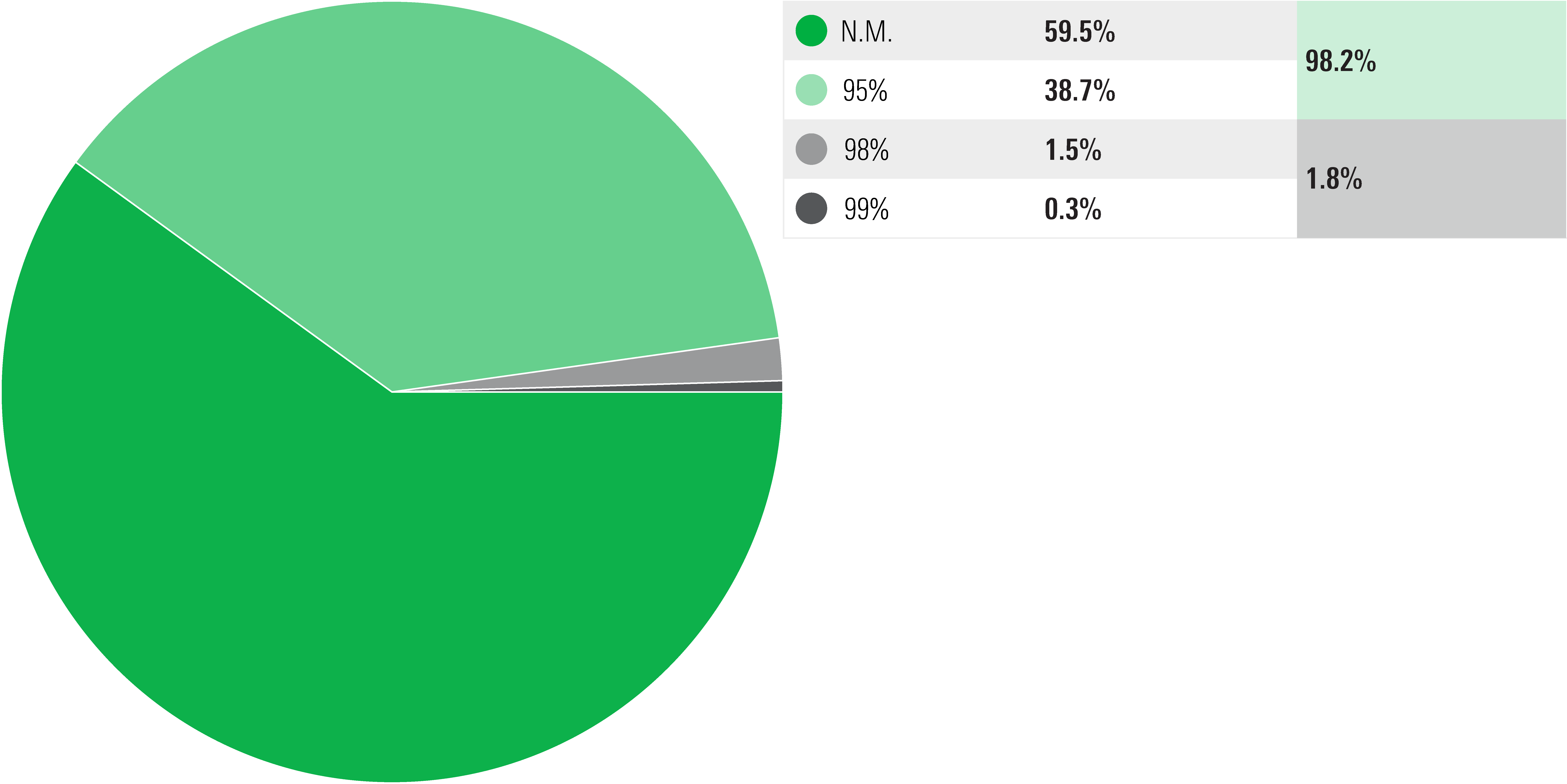
Only 1.8% of the valid funds reviewed are potentially closet indexing. While more than 95% of the variation in returns of another 39% of funds can be explained by the factors, the threshold allows sufficient room for some active management. 

Managers may claim they can time the market to the upside and shield against the downside. If true, that’s worth paying for. Here’s how to test this claim.  

Treynor and Mazuy proposed one approach that closely resembles returns-based style analysis. (1)

This method regresses a fund’s excess returns on both the excess returns of the market and on its squared form. In a given time period 𝑡, for a fund 𝑓, market proxy 𝑚 and risk-free rate 𝑟_𝑐,𝑡, the model is given by: 

r_f,_t−r_c,t=𝛼+𝛽(r_m,t−r_c,t)+𝛾(r_m,t−r_c,t)²+𝜖_𝑡 

A statistically significant, positive 𝛾 indicates market timing ability. A statistically significant negative 𝛾 would indicate that the manager times the market in the wrong direction. 

The data set needed for this analysis is the same as above. In fact, for this model, you don’t need any factors beyond the excess market returns. 

Start by squaring the excess returns. 

INPUT

ms_dataset['Excess_sq'] = ms_dataset['Excess'] ** 2 

Create lists to store results. 

INPUT

good_timers = [] 

bad_timers = [] 

no_ability = [] 

Next, fit the regression models. 

INPUT 

formula_rhs = "Excess + Excess_sq" 

model_fit = [] 

for fund in tqdm(valid_funds): 

    model = smf.ols(formula=f"{fund} ~ {formula_rhs}", data=ms_dataset).fit() 

    # Only for well fitted models, evaluate timing 

    if model.f_pvalue < 0.05: 

        model_fit.append(fund) 

        # Evaluate only highly significant results 

        if model.pvalues.loc['Excess_sq'] < 0.05: 

            if model.params.loc['Excess_sq'] > 0: 

                good_timers.append(fund) 

            else: 

                bad_timers.append(fund) 

        else: 

            no_ability.append(fund) 

    else: 

        continue 

Here’s how to visualize the findings. 

INPUT

abels = 'Good Timing', 'Bad Timing', 'No Ability' 

sizes = [len(good_timers), len(bad_timers), len(no_ability)] 

fig, ax = plt.subplots() 

explode = (.1, .1, 0) 

ax.pie(sizes, labels=labels, explode=explode, colors=plt.get_cmap("tab20").colors[:4],autopct='%1.1f%%') 

plt.show() 

OUTPUT

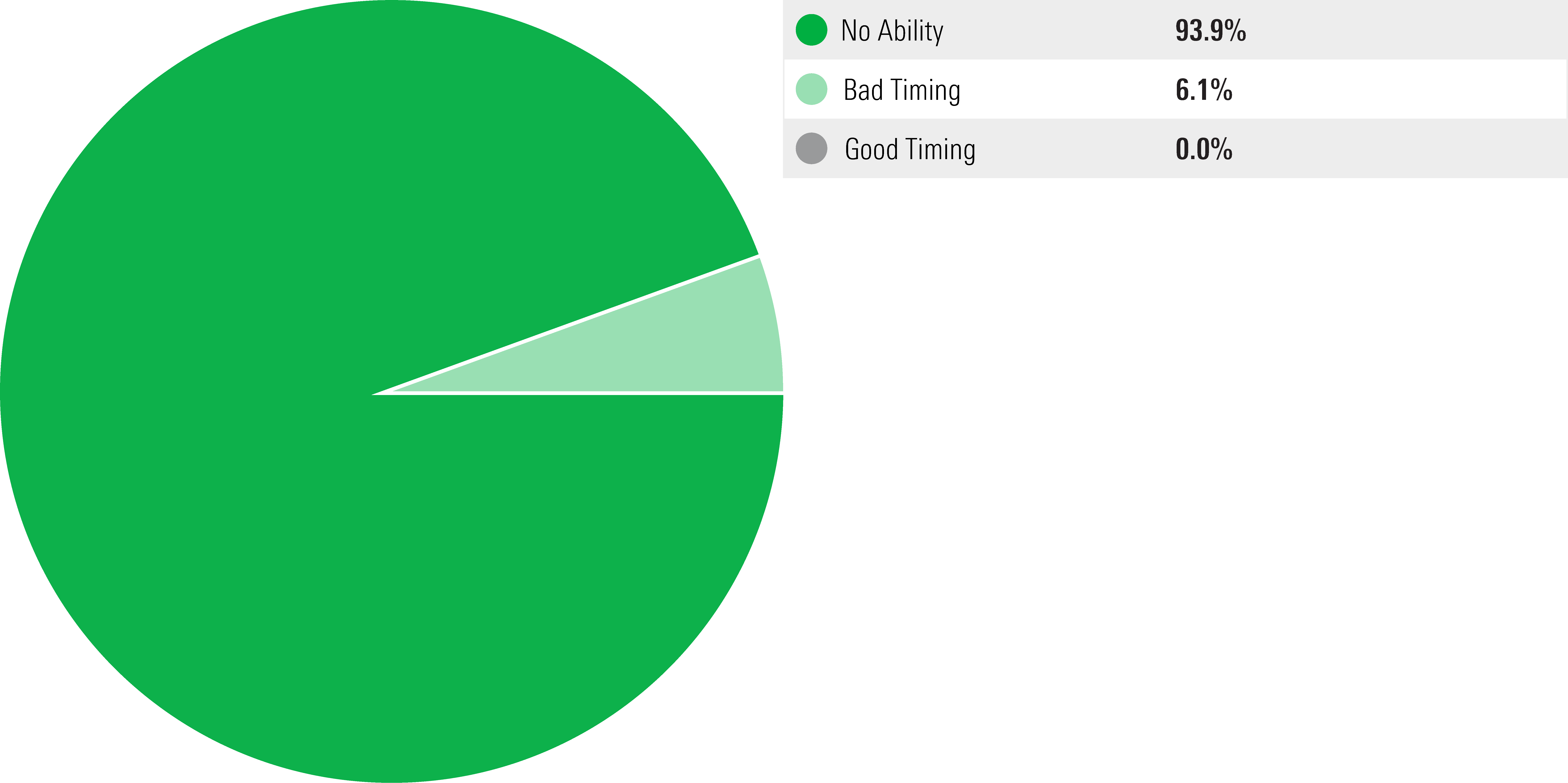
A poor result for proponents of active management.  

According to this analysis, 94% of management teams have no market timing ability. The remaining 6% have significant market timing ability, but in the wrong direction. These funds increased their exposure to the market when it was declining and reduced market exposure during periods of growth. 

This result would suggest that even if investors wish to buy expensive actively managed funds to access managerial skill, they should know that market timing isn’t a significant component of that skill. 

While these results are valid, please supplement them with deeper dives into holdings and other analyses before drawing conclusions about management strategies. One option is to perform rolling regressions over time and examine whether the results are consistent through time. 

With these code snippets, investment teams can make informed decisions about fund managers. These tips should give technical users more flexibility to customize analysis and manipulate data their way. 

Looking for more ways to use Python for style analysis? The complete guide includes additional case studies, examples, and code snippets.