Investment Style Analysis: Python Snippets for Evaluating Style Drift

Investors choose funds in the hopes that they align with their risk preferences and long-term goals. If funds drift from their stated intentions, investors could end up lost at sea. Funds need to follow their stated investment philosophy and process, even in unfavorable markets. 

Style analysis is the process of assessing investment philosophy. The quantitative approach can help you interpret how funds are likely to behave. Make informed comparisons and build diversified portfolios with accurate pictures of funds. 

Copy and paste these Python snippets to kickstart style analysis. For more real-life case studies and examples, download the style analysis guide.

Returns-based style analysis uses historical performance to calculate and show an investment’s composition, style drift, and relative performance against a benchmark.  

Returns-based style analysis is widely used due to its relatively light input data requirements. All you need are fund returns and premia for the style factors you want to evaluate. This type of regression analysis is sometimes called time series regression since the observations, or records, used for regression are sampled through time.

To conduct style analyses, you need two core categories of data. 

• Fund returns: Total return time series for the funds being analyzed. 

• Style factor data: Exposure and style premia. 

While many providers offer historical returns data, here we’ll connect to the Morningstar_data Python package to fetch data and statsmodels Python package for regressions. 

The Morningstar_data Python package gives data scientists, quants, and engineers convenient access to Morningstar data and the flexibility to use it in their preferred coding environments. To use the Python package, start by logging into Analytics Lab to retrieve your authentication token. Access full instructions on the developer site.

INPUT 

# testing_morningstar_data.py 

import os 

import morningstar_data as md 
 
os.environ['MD_AUTH_TOKEN']="paste copied token here" 

md.direct.get_morningstar_data_sets() 

import pandas as pd 

import statsmodels.formula.api as smf

First, fetch the data needed for style analysis of equity funds. Obtain the unique tickers for the funds you plan to analyze. Use the investments() function that searches for matching securities based on a keyword.

In this case, the keyword will be known ticker values. As an example, we’ll use SPY and MTUM. For each ticker, find the top five keyword matches in the Morningstar database and store the top match in a list. Then convert the list to a dataframe for review.

INPUT 

mstar_security_info = [] 

for t in tickers: 

    matches = md.direct.investments(keyword=t, count=5, only_surviving=True) 

    mstar_security_info.append(matches.head(1))  

security_df = pd.concat(mstar_security_info, axis=0) 

security_df 

OUTPUT 

If you can’t find the perfect matches on the first try, iterate the process. Going forward, use the SecId field.  

Next, pull 60 months of returns for these funds. We’re using the Morningstar data package here. 

INPUT 

fund_returns_raw = md.direct.get_returns( 

    investments=security_df['SecId'].tolist(), 

    start_date='2019-06-30', 

    end_date='2024-05-31' 

) 

fund_returns_raw.head(3) 

OUTPUT 

 Pivot these returns so that you can later join them with the factor premia, using the dates as keys.

INPUT 

fund_returns_wide = ( 

    fund_returns_raw 

    .pivot( 

        index='Date',  

        columns='Id',  

        values='Monthly Return' 

    ) 

    .div(100) 

) 

fund_returns_wide.head(3) 

OUTPUT

The second ingredient for returns-based style analysis is the set of factor premia. The Fama-French Three-Factor Model incorporates, as the name suggests, three factors: 

• Small minus big, or excess returns of small-cap companies over large-cap companies. 

• High minus low, or excess returns of value stocks with a high book-to-price ratio over growth stocks with a low book-to-price ratio. 

• Market risk premium, or portfolio return less the risk-free rate of return. 

The factor premia for this model are available in Prof. Kenneth French’s data library. Use the monthly North American three-factor premia. 

While you could get this data directly from the website and manipulate it with Pandas, the more convenient option is pandas-datareader. 

INPUT 

ff_premia = ff_premia_raw[0].div(100) 

ff_premia.index = pd.to_datetime(ff_premia.index.to_timestamp()) + pd.tseries.offsets.MonthEnd() 

ff_premia = ff_premia.rename(columns={'Mkt-RF': 'Market'}) 

ff_premia.head(3) 

OUTPUT

The Morningstar North America Equity Risk Model captures risk premiums across the region. The model considers additional factors like: 

• Liquidity, or how well a fund can meet cash flow demands. 

• Volatility, or variations in returns. 

• Yield, or the income generated by an investment. 

• Quality. High-quality firms have high profitability and low financial leverage. 

Here, use the monthly factor premia from the Morningstar North American Risk Model. These are available in the Risk Model tab in Morningstar Direct.

INPUT 

mstar_premia_raw = pd.read_csv('mstar-NA-premia.csv') 

mstar_premia_raw.head(3) 

OUTPUT

Format to set the date as index and decimalize by dividing by 100. 

INPUT 

mstar_premia = ( 

    mstar_premia_raw 

    .assign(Date=lambda x: pd.to_datetime(x.Date)) 

    .set_index('Date') 

    .div(100) 

) 

mstar_premia.head(3) 

OUTPUT 

In the Fama-French model, funds returns in excess of the risk-free rate are the endogenous variable, or the variable determined by its relationship to other variables in the model. Create the two independent variables first. 

First, fetch the available fund return dates, available premia dates, common dates, and risk-free rate. 

INPUT 

fr_idx = fund_returns_wide.index 

ff_idx = ff_premia.index 

cd = fr_idx.intersection(ff_idx) 

rfr = ff_premia.loc[cd, 'RF'] 

Now create the excess returns dataframe. 

INPUT 

fund_returns_excess = fund_returns_wide.sub(rfr, axis=0) 

Create a combined dataset. 

INPUT 

ff_dataset = fund_returns_excess.join(ff_premia, how='inner', validate='1:1') 

ff_dataset.head(3)

OUTPUT 

Now perform the regression. 

INPUT 

spy_ff = smf.ols(formula="FEUSA00001 ~ Market + SMB + HML", data=ff_dataset).fit() 

mtum_ff = smf.ols(formula="F00000PF2S ~ Market + SMB + HML", data=ff_dataset).fit() 

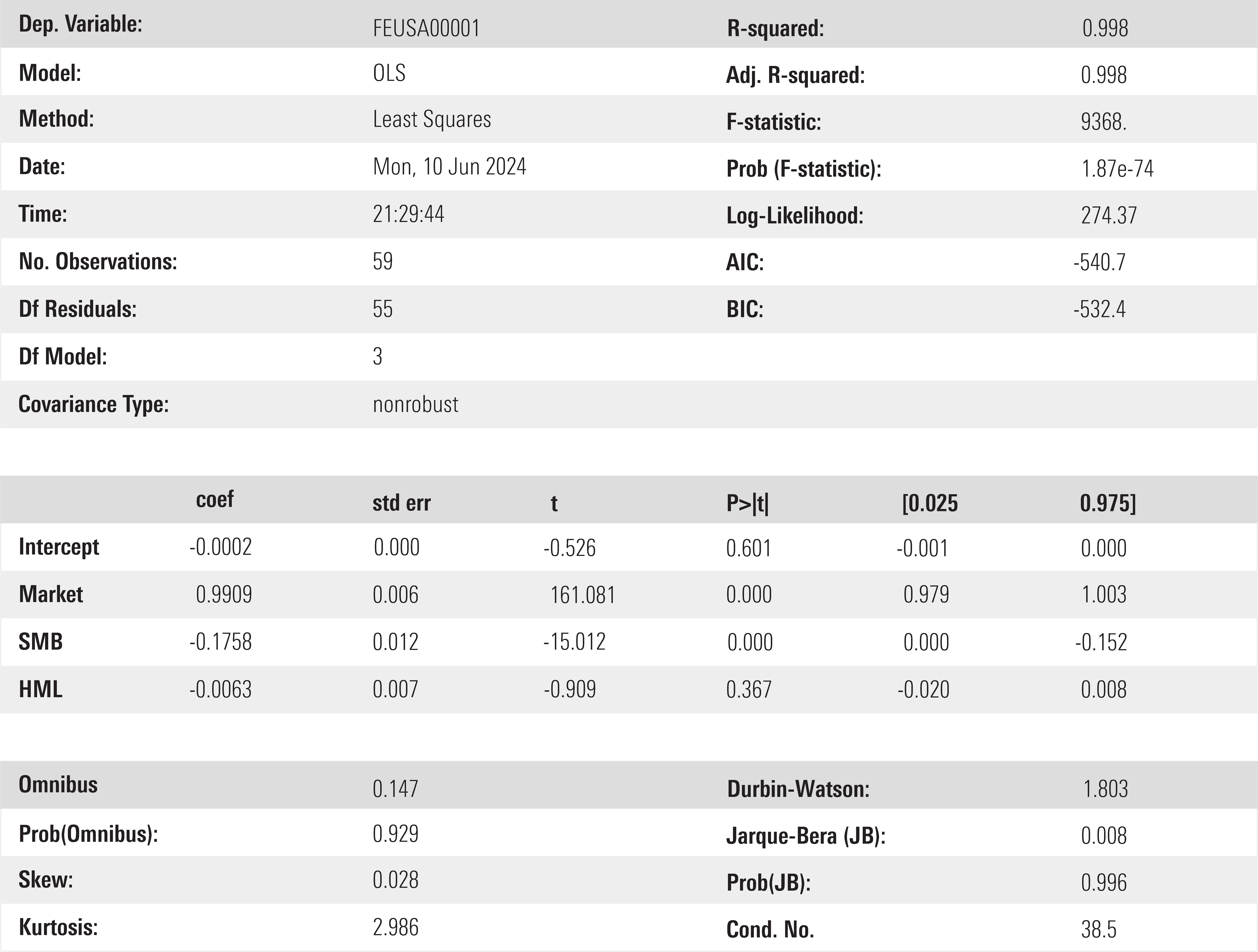
With the models trained, let’s examine the outcomes beginning with the first fund in our earlier list: SPY.  

As an S&P 500 index tracker, this fund should mimic the market since the S&P 500 is so often used as the definition of the market. However, since the fund and the index are decidedly large-cap, this size factor should show up in the factor exposures as well. 

Interpret the regression results just like any other multiple linear regression output.  

• Metrics such as the F-statistic and Adjusted R-squared represent the overall strength of fit of the model. 

• Gauge the statistical significance of individual coefficients with their t-stats or p-values. 

INPUT 

spy_ff.summary() 

OUTPUT: OLS Regression Results

No surprises here.  

The SPY ETF has a highly significant exposure to the market and SMB factors and an insignificant alpha and HML exposure. This makes sense since the fund has a blend style and explicitly tracks the index. If anything, the analysis could have shown a negative alpha equal to the fund’s expense ratio. 

Now let’s examine the results for MTUM, the iShares MSCI Momentum Factor ETF.  

As per the fund description, the fund attempts to invest in large- and mid-cap US-based companies with relatively high price momentum. While momentum is widely considered a factor, it’s not included in the Fama-French model.  

The MTUM results should show significant exposures to the market and possibly negative and significant exposures to SMB since the fund invests in larger companies. If the momentum and style factors happened to be correlated over the past five years, you might observe an incidental loading to style.  

In fact, you might observe a statistically significant alpha value in this model. 

INPUT 

mtum_ff.summary() 

OUTPUT

Note: Standard errors assume that the covariance matrix of the errors is correctly specified. 

The overall model is still a good fit based on the extremely significant p-value for the F-statistic. However, the R-squared of about 82% for this model is comparatively lower than the R-squared for the SPY model of about 99%.  

While those models could explain nearly all the variation in the fund returns, this model cannot account for about 20% of the variation. 

The only statistically significant exposure is to the “market” factor. Despite omitting small-cap stocks, the fund does not have a significant SMB loading. The coefficient is directionally correct with the negative sign but is not statistically indistinguishable from zero. 

With our risk model, you can evaluate exposure to other commonly accepted factors, such as momentum. Like before, fit the regression model to the factors in the Morningstar NA Equity Risk Model. 

Fetch the available fund return dates, available premia dates, common dates, and risk-free rates. 

INPUT 

fr_idx = fund_returns_wide.index 

ms_idx = mstar_premia.index 

cd = fr_idx.intersection(ms_idx) 

rfr = mstar_premia.loc[cd, 'Cash'] 

Now create the excess returns dataframe. 

INPUT 

fund_returns_excess = fund_returns_wide.sub(rfr, axis=0) 

Then create the excess market return column in the LHS. 

INPUT 

mstar_premia['Market_excess'] = mstar_premia['Market'] - mstar_premia['Cash'] 

Create a combined dataset. 

INPUT 

ms_dataset = fund_returns_excess.join(mstar_premia, how='inner', validate='1:1') 

Finally, perform the regression. With the statsmodels formula API, you can manipulate the formula like any other string. 

INPUT 

formula_rhs = "Market_excess + Size + Style + Yield + Volatility + Momentum + Quality + Liquidity" 

spy_ms = smf.ols(formula=f"FEUSA00001 ~ {formula_rhs}", data=ms_dataset).fit() 

mtum_ms = smf.ols(formula=f"F00000PF2S ~ {formula_rhs}", data=ms_dataset).fit() 

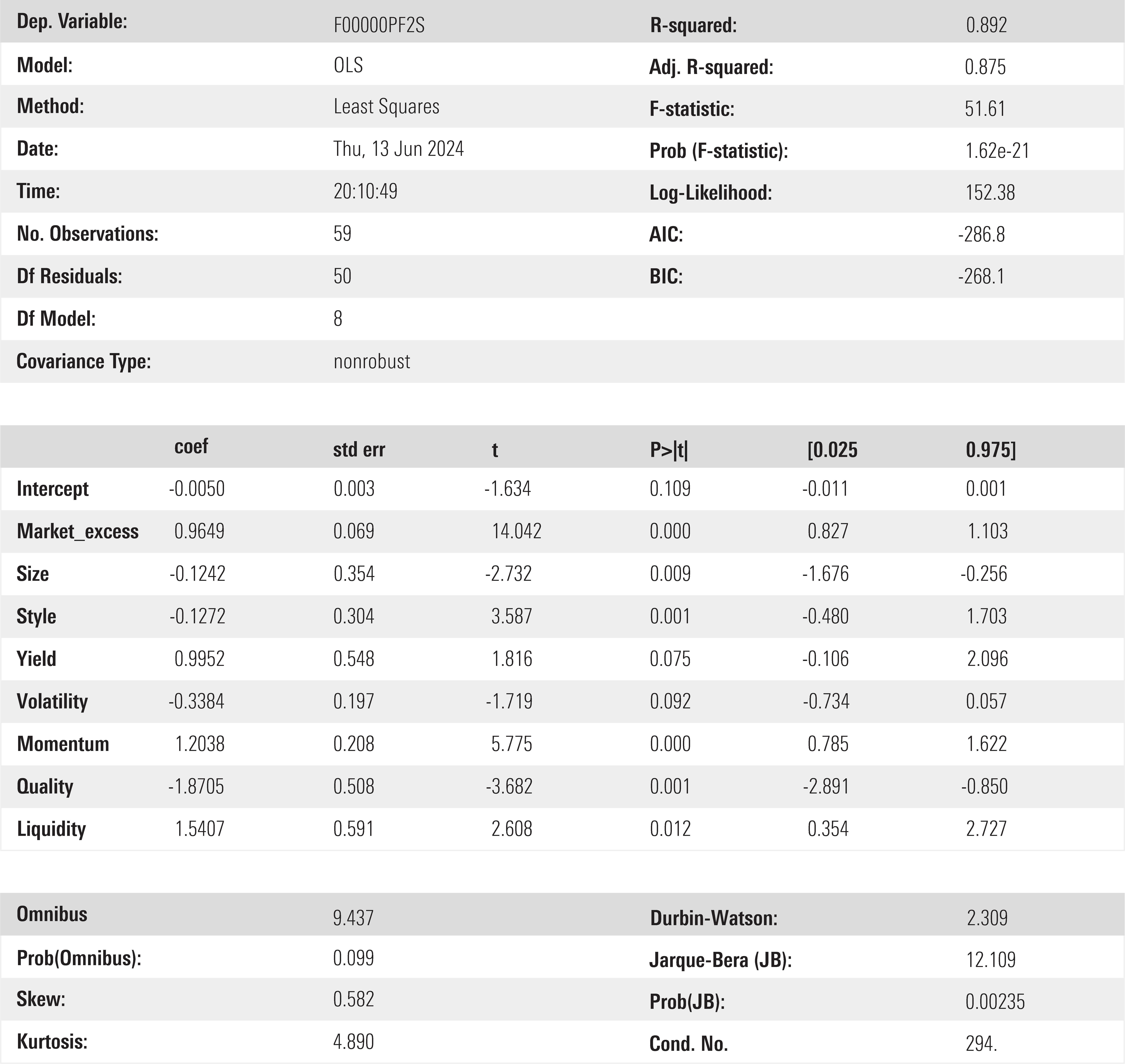
This time, let’s begin by analyzing MTUM. This fund’s investment objective says that it seeks to track stocks showing relatively higher price momentum. We expect to see a significant positive loading on the momentum factor. 

INPUT 

mtum_ms.summary() 

OUTPUT: OLS Regression Results

Note: Standard errors assume that the covariance matrix of the errors is correctly specified. 

These results reveal a few key differences from the Fama-French model analysis. 

The overall model is a good fit as judged by the F-statistic. The adjusted R-squared, which accounts for the increase in regressors, is also higher than before. This model can explain about 90% of the variation in fund returns. This is 10% more than earlier. 

As expected, the fund shows significant positive exposures to both the market and the momentum factors. You’ll also find a statistically significant negative loading to the size factor, which was expected due to the fund’s bias towards larger stocks. 

There are also statistically significant exposures to style and quality. These are incidental—the fund doesn’t explicitly attempt to capture these factor premia. But portfolio managers should be aware of these exposures so they can adjust the overall portfolio to account for them. 

Style analysis provides an objective lens for many useful tasks: 

• Evaluating funds. 

• Identifying unintended risks. 

• Optimizing intentional style tilts. 

• Arming investment teams with robust performance attribution insights. 

By measuring style exposure, you can ensure portfolios stick to their defined investment philosophies and processes. 

If you’re ready to dig into more advanced applications, the full guide contains more code snippets and case studies.